UPDATE: See the bottom of this post for new, higher definition, full-colour fractals!

While messing around with factorials, I stumbled across some unexpected and elegant fractal images.

As you probably know,  the factorial function n! is calculated by multiplying all the positive integers from 1 to n:

n! = 1 × 2 × 3 × … × (n − 1) × n

The function grows very quickly:

1! = 1
2! = 2
3! = 6
4! = 24
5! = 120
…
10! = 3628800
…
20! = 2432902008176640000
…
50! = 30414093201713378043612608166064768844377641568960512000000000000

Obviously, applying the factorial function more than once* just makes the sequence grow even quicker:

1!!  = 1
2!! = 2
3!! = 720
4!! = 620448401733239439360000
5!! = 6689502913449127057588118054090372586752746333138029810295671352301633557244962989366874165271984981308157637893214090552534408589408121859898481114389650005964960521256960000000000000000000000000000
…
10!! = Something with 22228104 digits
…
20!! = Something whose number of digits has 20 digits
…
50!! = Something ludicrously enormous

Clearly, unless we start with 1 or 2 (which will stubbornly stay the same no matter how many exclamation marks we stick to them), taking repeated factorials of a positive integer is not likely to achieve anything other than giving us (and our calculator) an almighty headache.

However, factorials are not limited to the positive integers. They can be extended to all real and complex numbers using something called the Gamma function. For example, it turns out that:

1.5! ≈ 1.329
(−1.5)! ≈ −3.545
i! ≈ 0.498 − 0.155i

OK, we still cannot take the factorial of a negative integer (we get “complex infinity”), but we have definitely got considerably more scope than we had when we were stuck with the naturals. Most interestingly, many of these new numbers do not become ridiculously large (or do nothing) as you take repeated factorials:

(1 − i)!     ≈ 0.653 − 0.343i
(1 − i)!!    ≈ 0.857 − 0.054i
(1 − i)!!!   ≈ 0.947 − 0.017i
(1 − i)!!!!  ≈ 0.978 − 0.006i
(1 − i)!!!!! ≈ 0.991 − 0.003i
…

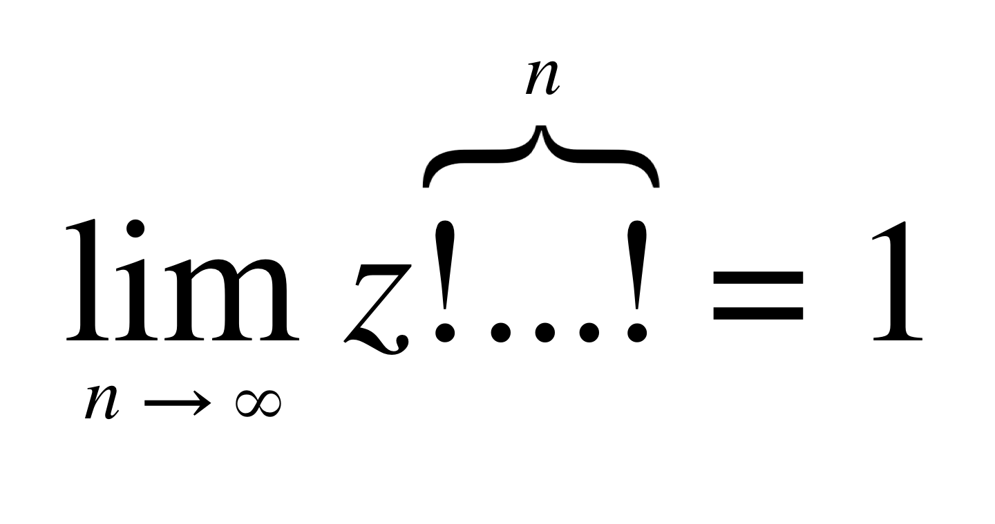
In this complex example, the imaginary part of our answers seems to be withering away and it looks like we are converging towards 1.

In fact, as far as I can tell, when taking repeated factorials, barring some extremely rare cases (solutions of z! = z) every complex number EITHER tends to 1 (like 1 − i, above) OR grows without limit (like all the positive integers greater than 2).

Let’s look at which complex numbers grow (diverge) under repeated factorialisation and which ones head for 1 (converge).** One way of visualising these two sets is to colour the complex plane, using one colour (say, white) for points that diverge and another colour (say, blue) for those that converge.*** If we wanted to be technical about it, we could say that the blue points represent the set of all z ∈ ℂ, such that:

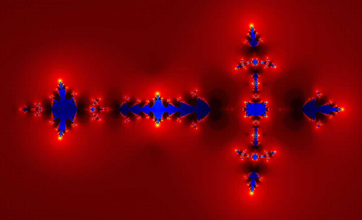
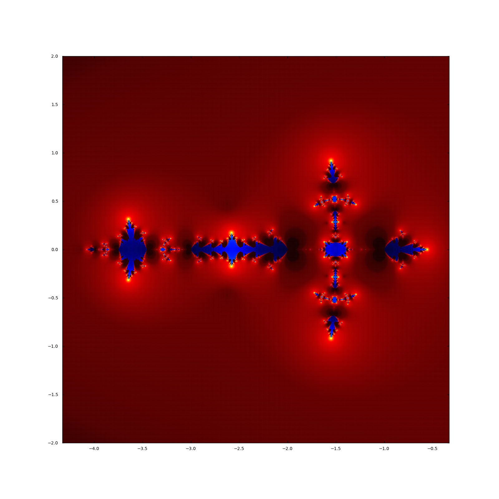
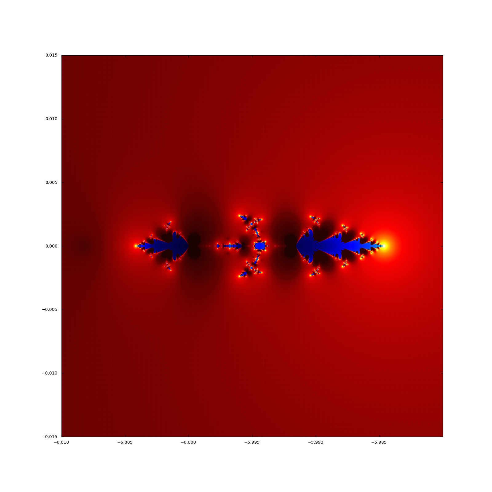
Anyway, using this procedure, some beautiful fractal patterns (patterns that are reproduced at smaller and smaller scales) start to emerge.**** For example, here is a section of our coloured-in complex plane around the negative real axis (CLICK ON IMAGES TO ENLARGE), exhibiting a fragile looking cruciform pattern:

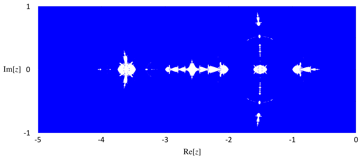
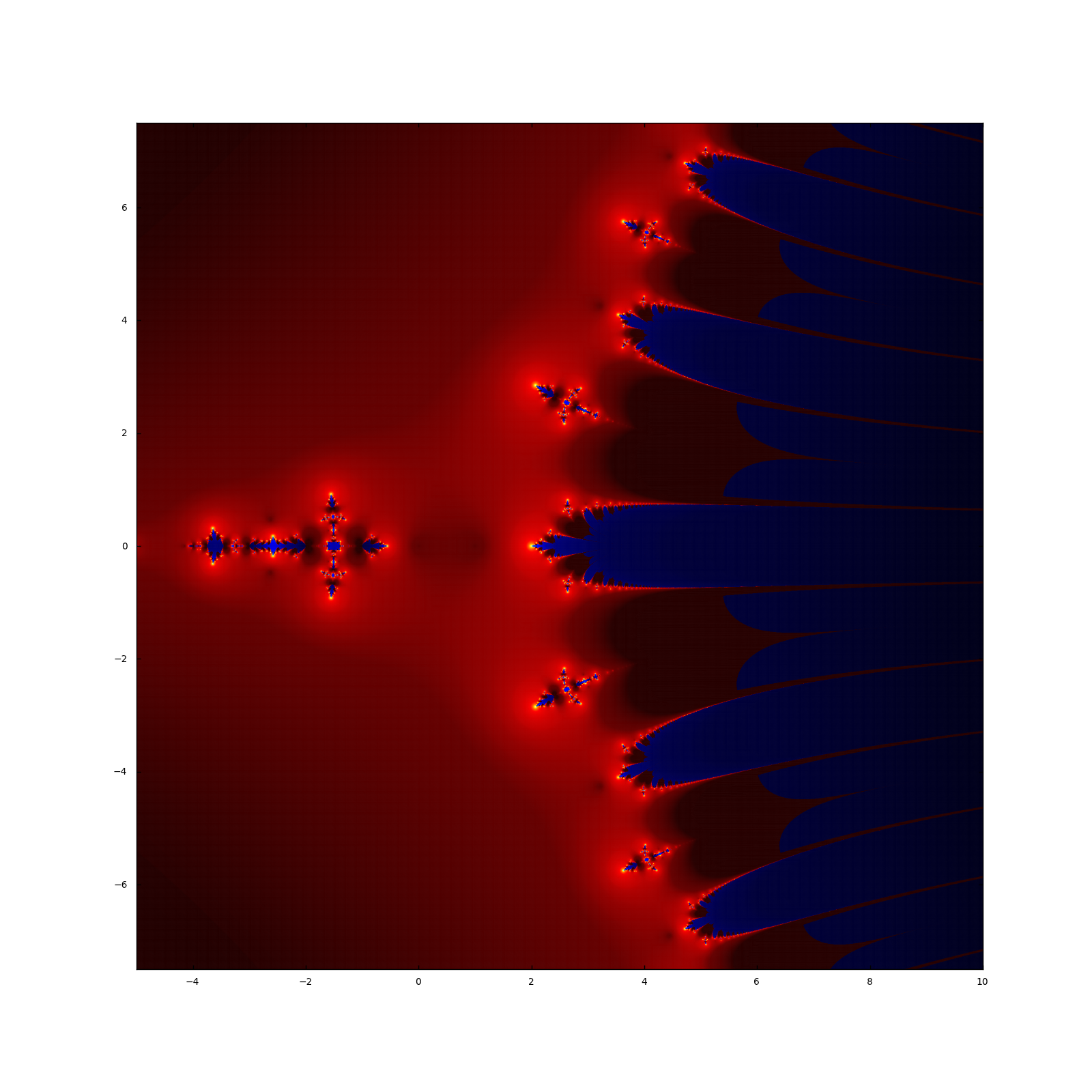
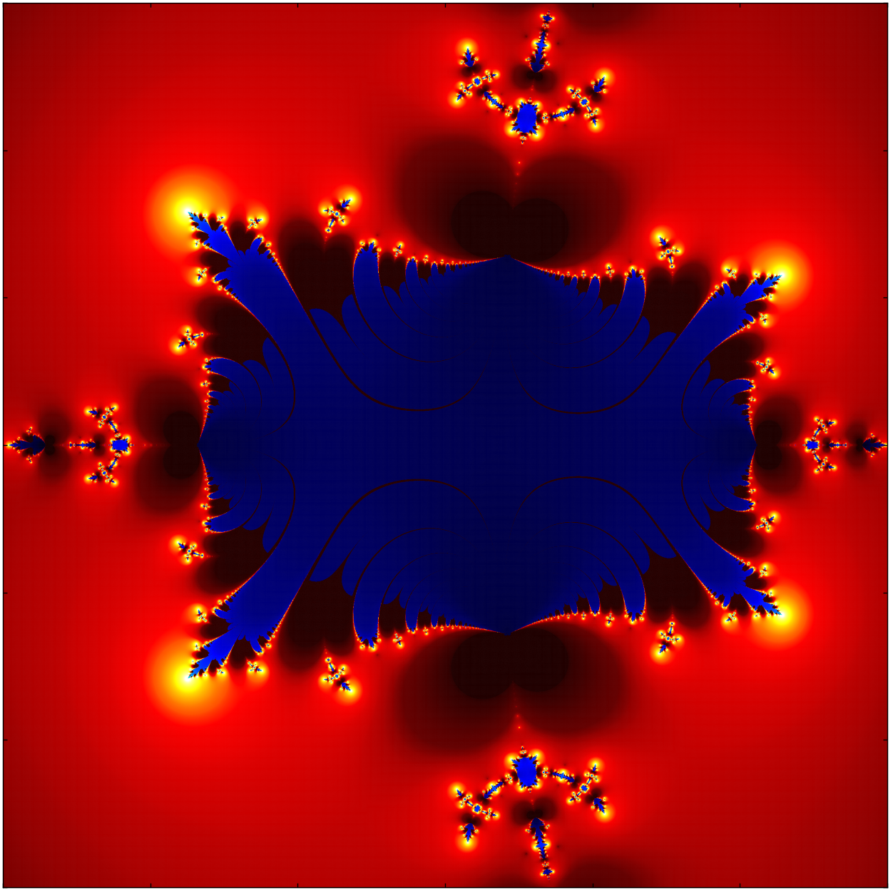
And here is a larger section around the positive real line:

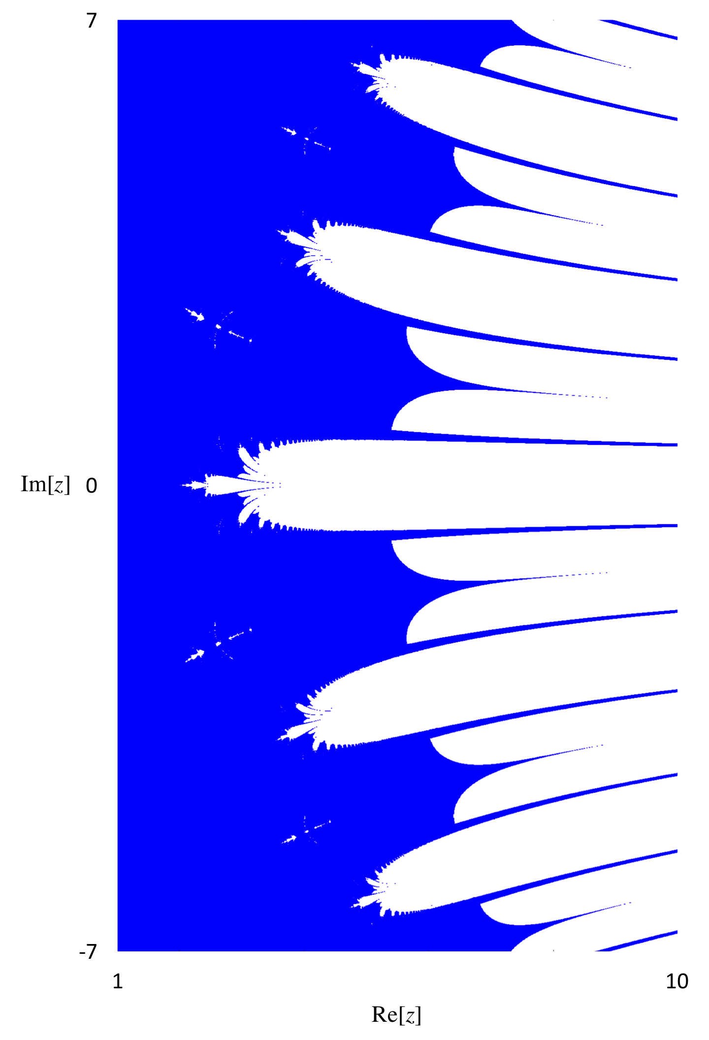
This vertical wall of self-similar warty protuberances seems to curve off to infinity above and below, separating the blue region to the left (where most points converge), from the white region on the right (where most points diverge). However, those blue filaments that can be seen heading out of the plot and deeper into the white region, may well also be making their way to infinity (in the positive real direction).

Smaller copies of the cruciform shape from the first plot can be seen swimming off between the protuberances. Vice versa, if you go back to the first image, you can just make out some of these protuberances reproduced on smaller scales in parts of the cruciform.

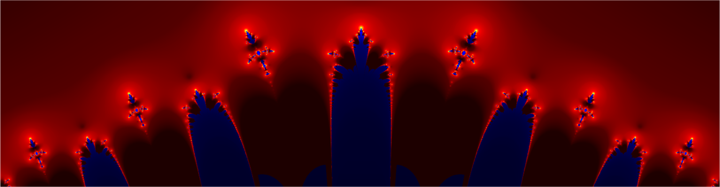
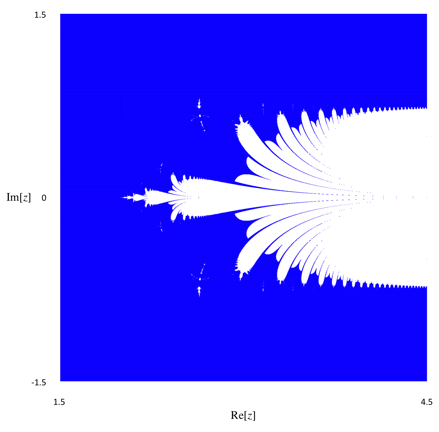
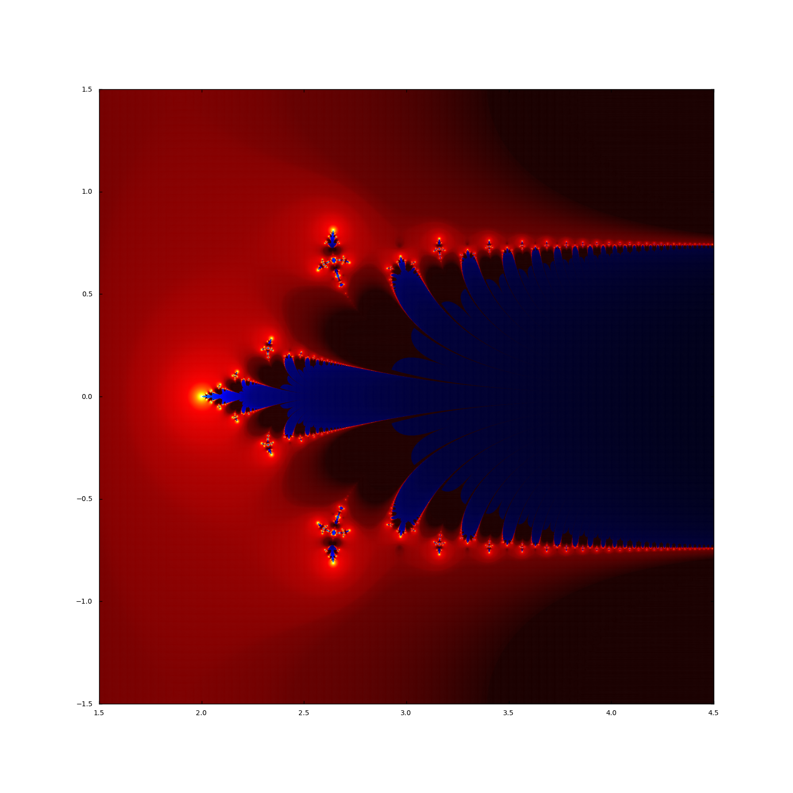
Here is a close up of the central protuberance in the second plot, in which you can see the distorted fractal structure in more detail.

I was not aware of these fractals, though I assume that they must have been observed before. A rather nice thing to stumble across, nonetheless!

---

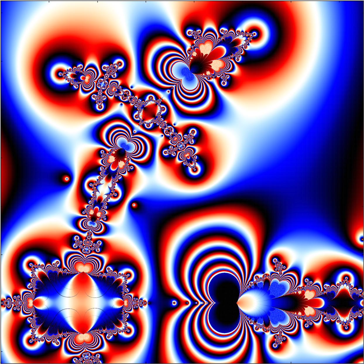
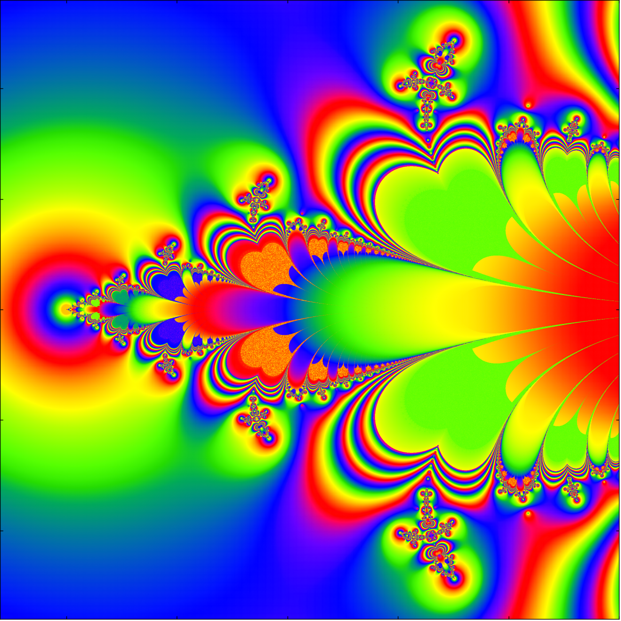
UPDATE: Here are some more colourful, higher definition images of these fractals. The convergent region is coloured from dark red (rapid convergence to 1) to yellow (slow convergence). The divergent region is coloured from dark blue (rapid divergence to infinity) to pale green (slow divergence).

Click on the images for full size versions, then click again to zoom to full size:

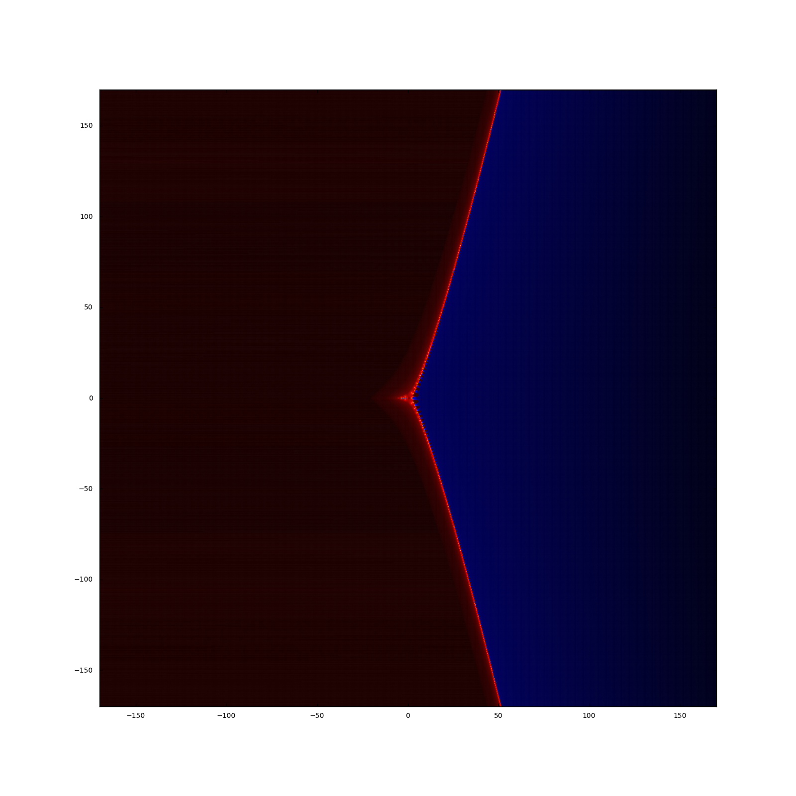
This first image shows more-or-less the widest possible scale that I could manage, for complex numbers with real and imaginary parts lying between −170 and +170. Numbers with imaginary parts any larger than that are too large for even an initial application of the factorial function in Python, so it is impossible to check whether they converge or not:

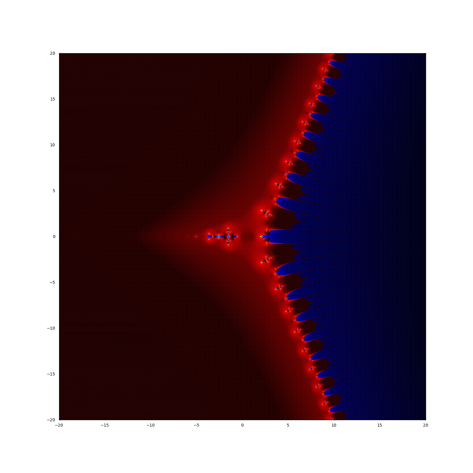
Let’s zoom in closer. Note the line of bright dots at unit intervals on the negative real (horizontal) line, behind the tail of the ‘cruciform’ shape. We will come back to these dots in a moment:

Here’s a still closer view:

And here’s a close-up of the central protuberance. Note that each of the little ‘swimmers’ emerging from the ‘coves’ between the sub-protuberances has its own set of trailing dots, like those behind the larger ‘cruciform’.

Here is the large ‘cruciform’ shape itself:

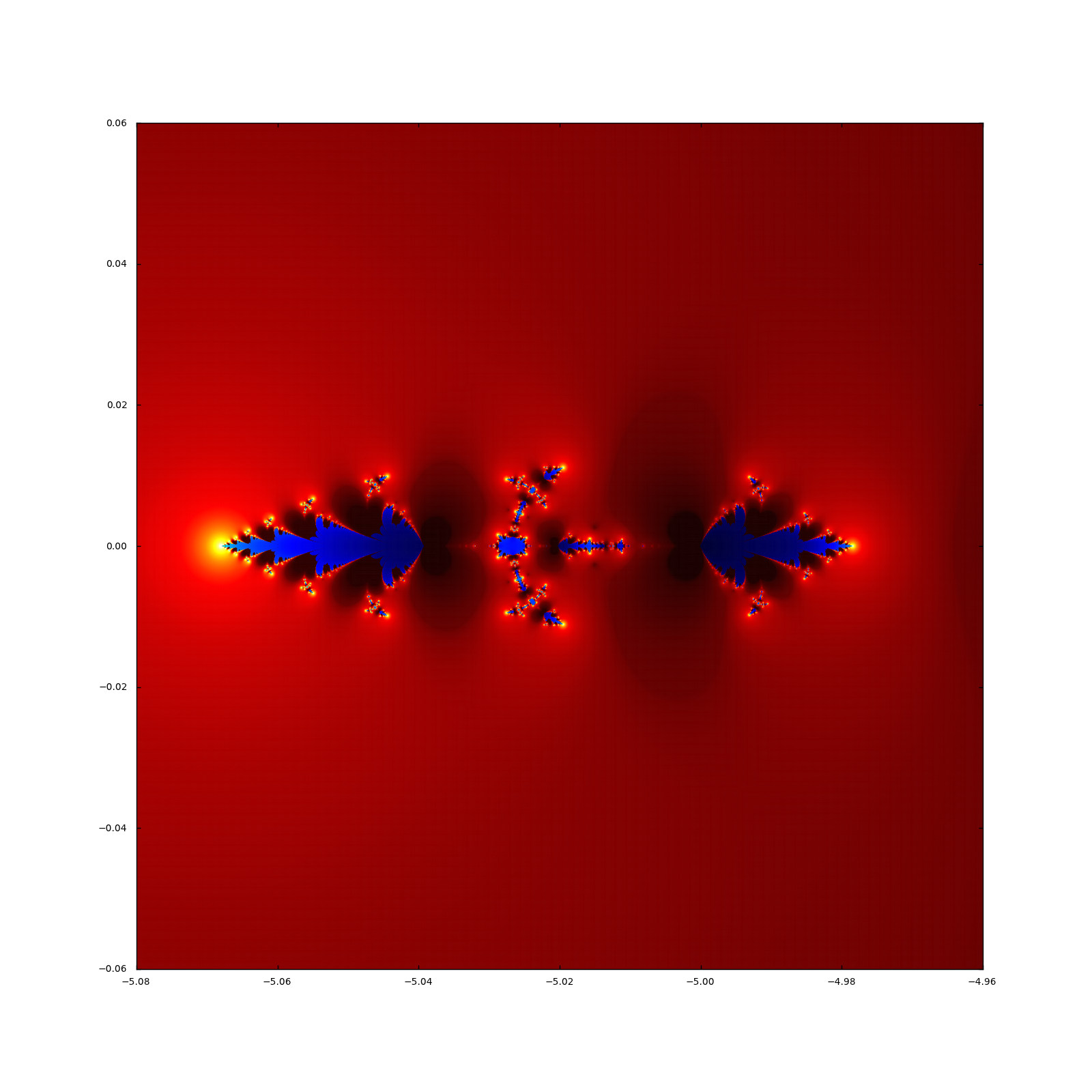
Now, back to those trailing dots that I mentioned earlier. This is what we see if we zoom in on the first of them (around -5 on the imaginary axis):

And this is the next one. Note that it is much smaller than the previous one (see the horizontal scale), but is otherwise a near mirror-image.

Zooming in to the island in the centre of the first of these “trailing dots”, you get a clearer view of the filament structure that runs through the blue regions:

The colouring is based on how many iterations were required before a number either got sufficiently close to 1 (the red/yellow regions) or became too large for Python to compute and was therefore inferred to diverge to infinity (the blue/green regions). This was then corrected by the final measurable size of the value when the convergence/divergence condition was triggered and some additional smoothing to produce continuous colours.

For each plot, the full range of the colour scheme is used, so the colours are not absolutely comparable between the images. This explains why the largest scale widest zoom image is mostly very dark.

Here are a couple of images with alternative colour schemes, just for fun:

 

A CAUTIONARY REMARK

I should say that, while I can be quite sure that values in the red region converge to 1, I cannot be at all sure that the dark blue region is genuinely divergent (with the exception of the positive real line). Perhaps after applying a number of factorials to the complex numbers in this region, they would actually crash back to 1, having passed through some unimaginably enormous values that the computer was unable to cope with. This is perhaps not all that unlikely, because those ‘red’ values in the figure that lie far from the real line do essentially behave in exactly this way.

Still, you should never let a pesky integer overflow get in the way of a pretty picture, right…?

---

* I see from Wolfram that using multiple factorial symbols (e.g. 9!!!!), technically denotes something called a multifactorial, rather that simply indicating multiple applications of the factorial function, as I intend. However, on the grounds that the correct notation (((9!)!)!)! is rather ugly, I am choosing to ignore this issue.

** I am pretty sure that we do not need to worry about the rare special cases, like z = 2, which converge to something other than 1. As far as I can tell, these are just the solutions of z! = z, which I believe to be sparse in the complex plane. In other words, although there are (I think) an infinite number of them, they do not take up any space, so we could not really colour them even if we wanted to.

*** This is the same principle that is used in visualising Julia Sets of rational complex functions.

**** The images were created in Python, using SciPy and Matplotlib.

---

Thomas Oléron Evans, 2015